Demo for Basic Usage
The python module imfits is developed for handling fits files easily. Here is a demo for the basic usage of imfits. The fits data used in this demo are all from Sai et al. (2020).
Read fits file
The base object of this module is the python class Imfits, which reads and contains data and header information of fits files. The below is an example for cube data.
[1]:
# import modules
import numpy as np
# if path is not set
#import sys
#sys.path.append('/PATH/TO/imfits')

from imfits import Imfits


# read cube
f = 'l1489.c18o.contsub.gain01.rbp05.mlt100.cf15.pbcor.croped.fits'
cube = Imfits(f)
print('Data dimension: %i'%cube.naxis) # Number of axes
print('Data shape: ', cube.data.T.shape) # Data are contained in 'data'
print('Axes: %s, %s, %s, %s'%tuple(cube.label_i)) # Each axis
The third axis is  FREQ
Convert frequency to velocity
Data dimension: 4
Data shape:  (400, 400, 69, 1)
Axes: RA---SIN, DEC--SIN, FREQ, STOKES
WARNING: FITSFixedWarning: 'datfix' made the change 'Set MJD-OBS to 57166.678867 from DATE-OBS'. [astropy.wcs.wcs]
WARNING: FITSFixedWarning: 'obsfix' made the change 'Set OBSGEO-L to   -67.754929 from OBSGEO-[XYZ].
Set OBSGEO-B to   -23.022886 from OBSGEO-[XYZ].
Set OBSGEO-H to     5053.796 from OBSGEO-[XYZ]'. [astropy.wcs.wcs]
You can call variables associated with the fits file. Basic variables are
data: Intensity as N dimensional ndarray.
xx, yy: RA and Dec offset coordinate grid for the FK4, FK5 and ICRS frames (deg).
xx_wcs, yy_wcs: Absolute WCS coordinate grid (deg).
xaxis, yaxis, vaxis and saxis: x, y, velocity (or frequency), and stokes axes (deg or km/s).
delx, nx: spacing and length of x axis. Same for y, v and s axes.
restfreq: Rest frequency (Hz).
beam: Beam size in a format of [bmaj, bmin, bpa] (in arcsec, arcsec and deg, respectively).
Imfits can also read the continuum data and the position-velocity (PV) diagram.
Draw maps
The drawmaps submodule from imfits makes it easy to plot maps of the fits data. Belows are a few examples.
Intensity maps
intensitymap from AstroCanvas can be used for an image with two spatial axes at a single frequency (e.g., continuum and moment maps). The simplest usage is as follows.
[2]:
# import module
from imfits import drawmaps as dm
# read file
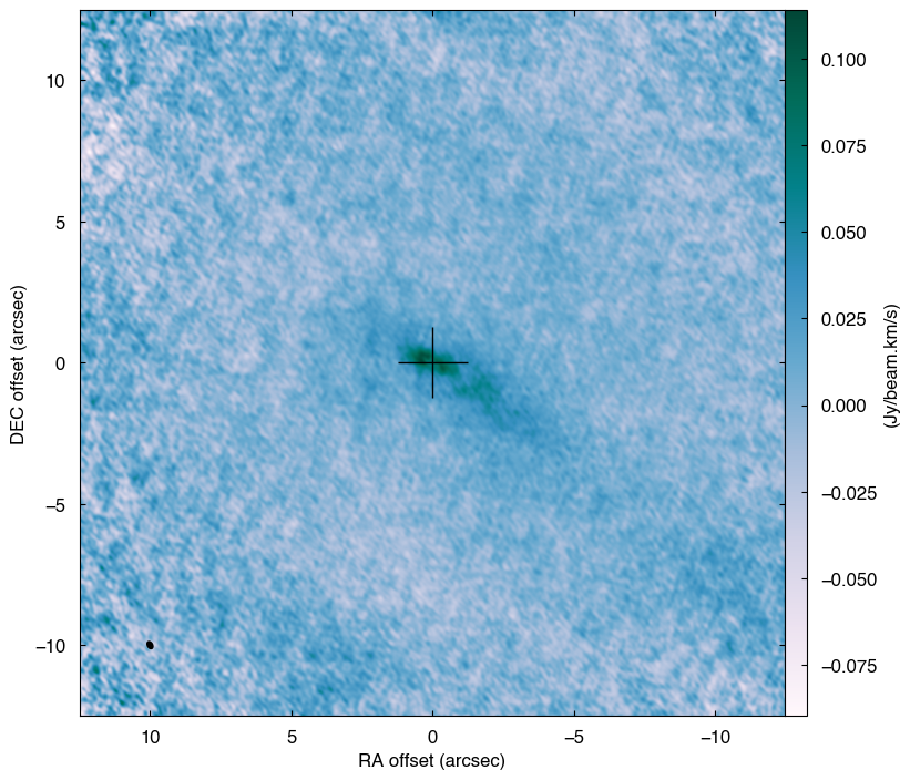
f = 'l1489.c18o.contsub.gain01.rbp05.mlt100.cf15.pbcor.mom0.trimed.fits' # moment zero map
im = Imfits(f)
# make plot
canvas = dm.AstroCanvas((1,1)) # Define a canvas where an image is plotted. Give (n_row, _col).
canvas.intensitymap(im)
plt.show()
WARNING: VerifyWarning: Invalid 'BLANK' keyword in header.  The 'BLANK' keyword is only applicable to integer data, and will be ignored in this HDU. [astropy.io.fits.hdu.image]
WARNING: FITSFixedWarning: 'datfix' made the change 'Set MJD-OBS to 57166.678867 from DATE-OBS'. [astropy.wcs.wcs]
CAUTION read_header: No keyword PCi_j or CDi_j are found. No rotation is assumed.
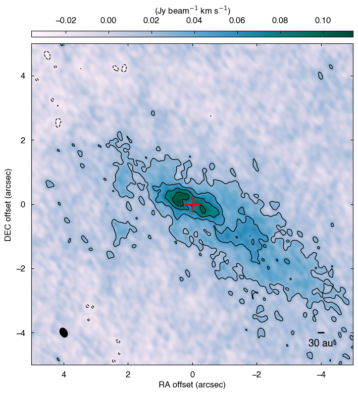
The map can be saved to a pdf file by canvas.savefig('filename'). More options can be given for more detailed plot settings.
[10]:
# rms of the map
rms = 8.e-3 # Jy/beam
# Define a canvas
canvas = dm.AstroCanvas((1,1))
# With more options
canvas.intensitymap(im,
                    imscale = [-5,5,-5,5], # map extent to show
                    color = True, # Add color
                    cmap = 'PuBuGn', # color map
                    contour = True, # Add contour
                    clevels = np.array([-3,3,6,9,12,15.]) * rms, # contour level
                    cbarlabel = r'(Jy beam$^{-1}$ km s$^{-1}$)', # color bar label
                    cbaroptions = ['top', '2%', '2%'], # colorbar options
                    ccross = True, # Add a cross at the center
                    prop_cross = [0.5, 2., 'r'], # Cross properties
                    scalebar = [30 / 140., '30 au', 'bottom right', 'k', 14] # Add a scale bar; [length in arcsec, text, location, color, font size]
                    )
plt.show()
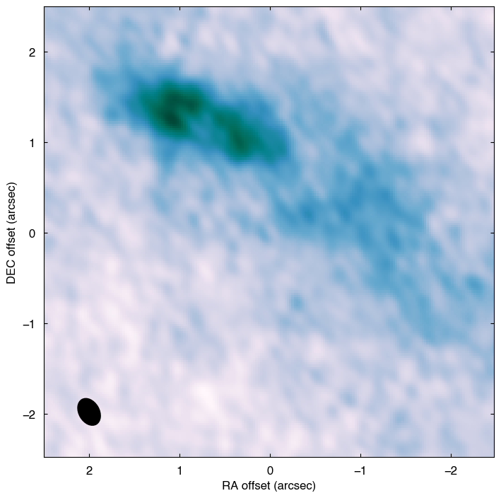
The data can be editted before making plots. Particularly, trimming data makes the plot speed much faster when the data size is huge.
[14]:
# fits file
f = 'l1489.c18o.contsub.gain01.rbp05.mlt100.cf15.pbcor.mom0.trimed.fits'
# new center
center = '4h4m43.02s 26d18m55s'


# read file
im = Imfits(f)
# shift map center
im.shift_coord_center(center)
# trim image
im.trim_data([-2.5,2.5], [-2.5,2.5]) # give xlim, ylim in arcsec


# plot
canvas = dm.AstroCanvas((1,1))
canvas.intensitymap(im, ccross=False, colorbar=False,)
plt.show()
WARNING: VerifyWarning: Invalid 'BLANK' keyword in header.  The 'BLANK' keyword is only applicable to integer data, and will be ignored in this HDU. [astropy.io.fits.hdu.image]
WARNING: FITSFixedWarning: 'datfix' made the change 'Set MJD-OBS to 57166.678867 from DATE-OBS'. [astropy.wcs.wcs]
CAUTION read_header: No keyword PCi_j or CDi_j are found. No rotation is assumed.
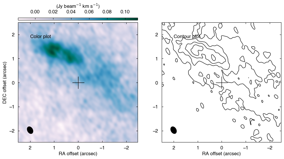
AstroCanvas is working like a wrapper of matplotlib.pyplot and contains a figure and axes of matplotlib. Therefore, by calling them, more flexible plots can be done.
[15]:
rms = 8.e-3 # Jy/beam

# two plots side by side
canvas = dm.AstroCanvas((1,2))
canvas.intensitymap(im,
                    iaxis=0, # index of panel
                    color=True, # color plot
                    contour=False, # contour plot
                    cbarlabel=r'(Jy beam$^{-1}$ km s$^{-1}$)', # color bar label
                    cbaroptions=['top', '2%', '2%'], # colorbar options
                    )
canvas.intensitymap(im,
                    iaxis=1, # index of panel
                    color=False, # color plot
                    contour=True, # contour plot
                    clevels=np.array([-3.,3.,6.,9.,12.,15.])*rms, # contour level,
                    cbarlabel=r'(Jy beam$^{-1}$ km s$^{-1}$)', # color bar label
                    cbaroptions=['top', '2%', '2%'], # colorbar options
                    )
canvas.axes[1].set_ylabel('') # off ylabel

# add something by yourself
ax1 = canvas.axes[0]
ax1.text(0.1, 0.9, 'Color plot',
       ha='left', va='top', transform=ax1.transAxes)
ax2 = canvas.axes[1]
ax2.text(0.1, 0.9, 'Contour plot',
       ha='left', va='top', transform=ax2.transAxes)

# save figure
#canvas.savefig('momentzero', ext='pdf')
# show
plt.show()
[ ]: