PV diagrams
Here, we present how to read and plot position-velocity (PV) diagrams with imfits. The simplest use is as follows:
[1]:
# import modules
import numpy as np
# if path is not set
#import sys
#sys.path.append('/PATH/TO/imfits')

from imfits import Imfits
from imfits.drawmaps import AstroCanvas


# read PV diagram
f = 'l1489.c18o.contsub.gain01.rbp05.mlt100.cf15.pbcor.croped.pv.fits'
pv = Imfits(f, pv=True) # Add the pv option

# plot
canvas = AstroCanvas((1,1))
canvas.pvdiagram(pv)

#canvas.savefig('pvdiagram', ext='pdf')
plt.show()
Convert frequency to velocity
More detalied settings can be given like the followings:
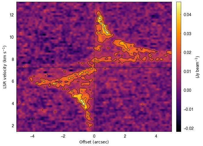
[2]:
rms = pv.estimate_noise()

canvas = AstroCanvas((1,1))
canvas.pvdiagram(pv,
                 color = True,
                 colorbar=True,
                 cmap = 'inferno',
                 contour = True,
                 clevels = np.array([-3,3,5,7,9])*rms,
                 x_offset=True, # offset for the horizontal axis
                 vsys=7.22, # systemic velocity
                 ln_var=True, # plot vertical center (systemic velocity)
                 ln_hor=True, # plot horizontal center (zero offset)
                 cbaroptions=('right', '3%', '3%'),
                 cbarlabel=r'(Jy beam$^{-1}$)')

plt.show()